
The 3D forward model
The interest in a new 3D forward model is to compare the solutions of various codes among each other but also to investigate how well the galvanic effects are dealt with in the current codes.
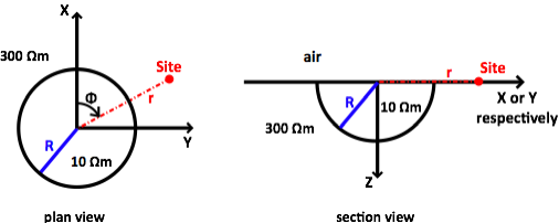
The 3D forward model consist of 10 Ωm hemisphere (radius R = 5 km) directly beneath the surface of a homogeneous 300 Ωm half-space (after Groom & Bailey, 1991). The centre of the hemisphere is defined as origin of the coordinate system.
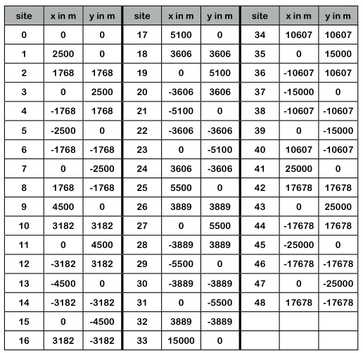
The figure below shows sketches of the section and plan view. The site locations are defined in Cartesian coordinates and listed in the table below.

One site is located in the centre of the hemisphere, all other sites are located on circles of different radii from the centre (inside and outside the hemisphere).
-
I.Please calculate the forward responses at all sites for the period range of 0.01 s to 10 000 s (0.01 s, 0.018 s, 0.032 s, 0.056 s, 0.1 s, 0.18 s, 0.32 s, ...., 5600 s, 10000 s).
-
Please email (marion@cp.dias.ie) the results as a plain ASCII format file with the following columns: x (in m), y (in m), period (in s), ρxx, Φxx, ρxy, Φxy, ρyx, Φyx, ρyy and Φyy. It is your responsibility to send the data using the correct coordinate system for the impedance (right-handed Cartesian with x pointing North, y pointing East and z positive downwards) and using the e+iωt sign convention for the time dependency. The kind of code (FD, FE, integral equation,...) you used, mesh dimensions and the computing time together with some properties (CPU speed, memory,...) of the used computer/cluster might also be interesting for comparison. It would be great if you could include a few words about that in your email.
-
-
II. Run an inversion of the 3D forward responses you calculated yourself (in I.)
Submitted forward responses will only be plotted and not check for possible different sign conventions or coordinates. Make sure you use the correct ones (e+iωt sign convention for the time dependency & for the impedance a right-handed Cartesian coordinate system with x pointing northwards).
Send your responses latest by 1st March 2011.
If you wish you can check your responses curves against the analytical solution of the galvanic limit given in Groom & Bailey, 1991 (Geophysics, 56, p. 496 - 518).

Dublin Institute for Advanced Studies, School of Cosmic Physics, 5 Merrion Square, Dublin 2, Ireland
Tel +353 - 1 - 6535147, Fax +353 - 1 - 443 - 0575, marion@cp.dias.ie
